Check this site for the Sussex
Univ online tutorial on major topics in auditory psychophysics.
<http://www.biols.susx.ac.uk/home/Chris_Darwin/Perception/Lecture_Notes/Hearing_Index.html>
Another good tutorial site is:
http://www.pc.rhul.ac.uk/courses/Lectures/PS1061/L5/PS1061_5.htm
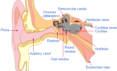
1. Anatomy and physiology of the ear.
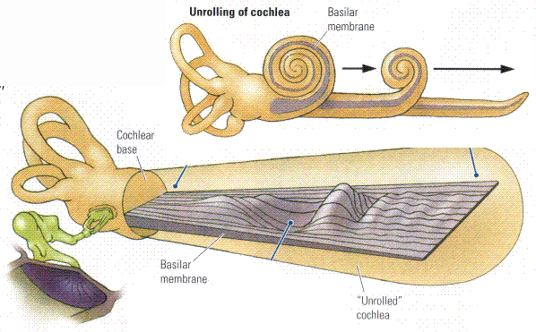
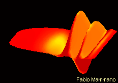
The BASILAR MEMBRANE (BM) is The spiral organ within the cochlea that mechanically separates frequency components of sound. Different frequencies cause local maxima in the amplitude of the travelling wave that moves down the basilar membrane at different locations. High frequencies get maximum response at the base (early) end of the cochlea (closest to the oval window). Perhaps surprisingly, the lower frequencies move farther up the BM. The lowest frequency with a unique location (at the very top end of the cochlea) is about 200 Hz. Thus frequencies below 200 Hz rely entirely on interpretation of time intervals.2. The Auditory Pathway
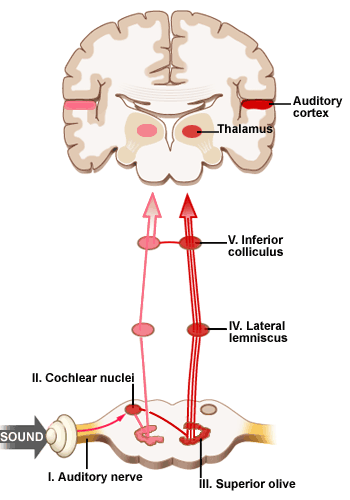
The ORGAN OF CORTI is a spiral structure lying along the full length of the basilar membrane which converts membrane motion into neural pulses. It is designed so that 4 rows of hair cells (one row of inner hair cells and 3 rows of outer hair cells) are mechanically disturbed by the passage of the sound wave along the BM. Each hair cell connects to a neuron that takes the signal to the central auditory system.
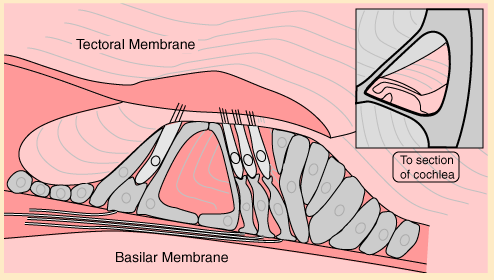
This is the sequence of nuclei in the brain stem leading from the cochlea to the auditory cortex in the superior temporal lobe of the cerebrum. The auditory nerve (or 8th cranial nerve) goes from the cochlear to
the cochlear nucleus which has a clear frequency map along its surface. The primary connections from each cochlear nucleus are to the opposite hemisphere. Each of the nuclei (the cochlear nucleus, superior olive, lateral leminiscus, inferior colliculus and thalamus) has a tonotopic map (ie, frequency-based map) but each also has cells that respond to increasingly complex patterns at higher levels. Some amount of lateral inhibition (that is, competition between regions) occurs at each level. At the higher levels the competition can amount to a `choice' between, eg, one syllable or another syllable.
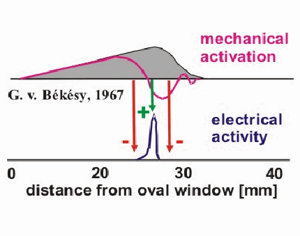
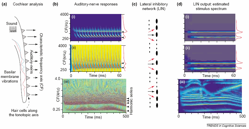
LATERAL INHIBITION. At a number of locations in the auditory system there are `frequency maps', that is, places where each cell in a sheet of cells responds maximally to input at a particular frequency and its neighbors in one direction respond to higher fs and in the other direction to lower fs. On such a map, if each nerve cell inhibits its neighbor in proportion to its own excitation, then a pattern that is blurry can be sharpened. For example, in the figure below the grey area represents the deflection of the basilar membrane by a midfrequency pure tone. Notice that all the hair cells in the grey region are disturbed and will fire.
But if in the cochlea itself or in the cochlear nucleus, cell A inhibits its neighbor, cell B, with value 4, and B inhibits A with value 6 (because it received more excitation), then very shortly A will slow down its firing but B will continue (unless inhibited by an even more active cell on the other side). Thus, if there is a whole field of these with each inhibiting its neighbors on both sides for a little distance, then only the most excited cell will inhibit both neighbors and remain active (as suggested by the plus and minus signs in the figure). Thus the lower dark curve of neural activity represents the pattern in the cochlear nucleus -- with only a narrow band of excitation at the frequency of the presented sinusoid. This is how the gross wave motion down the basilar membrane can be sharpened up so that the peak of envelope of membrane motion is picked out. Of course, we often need to hear more than one possible frequency so these neighborhoods of inhibition must be narrow. If you have a vowel with several independent formant frequencies, then there will be multiple local peaks of activity. Thus something that is fairly similar to a sound spectrum is produced along the frequency map of the cochlear nucleus. The spectra in column (b) in the figure below are transformed by lateral inhibition into the spectra of column (d).
PLACE CODING vs TIME CODING: As noted above, only frequencies above 200 Hz have unique maxima on the BM. This means that particular fibers in the auditory nerve are maximally active when their frequency is present in sound. The frequency at which a nerve fiber is most active is called its characteristic frequency or CF. But the mechanical action of the cochlea is such that frequencies below about also 4000 Hz are transmitted directly as waveforms into the auditory nerve. That is, for lower frequencies, the BM acts rather like a microphone translating mechanical pressure waves into waves of neural activation in time. This means that, between about 200 Hz and 4 kHz there is both a place code (where activity in specific fibers indicates teh frequency components in the sound) and a time code (where the temporal pattern of sound waves appears as a temporal pattern of fiber activation). Below 200 Hz, there is only a temporal representation of a wave, that is, the ear is not doing spectral analysis but only serving as a microphone to convert the mechanical pattern into a neural one.
The image below from Shihab Shamma (from Trends in Cognitive Science, 2001) shows the basilar membrane on the left (a) with computationally simulated auditory nerve representation of 3 patterns in (b). The top, (i), is a low intensity pattern of a 300 Hz plus a 600 Hz pure tone. Next, (ii), is the same tones but much higher intensity. The third is the phrase ``Right away'' (probably male talker). Column (c) suggests the lateral inhibitory network (in lower brainstem nuclei). Column (d) shows the simulated spectrogram available to the higher-level auditory system for analysis. Notice that both (bi) and (bii) look nearly identical in (d) (which is appropriate since they differ only in intensity).
For the speech example in (biii) notice that it is very difficult to interpret (even though several harmonics are pointed to by arrrows along the right edge), but in (diii), you can see at least 4 distinct harmonics in the low-frequency area, as well as F2, F3 and F4 (where the harmonics are merged). Notice the F3 sweep for the [r] of right and the F2 sweep for the [wej] in away. The display (diii) shows approximately the information available to the central auditory system, that is, to primary auditory cortex and other auditory areas. Clearly it resembles a traditional sound spectrogram except that the lower frequency region looks like a `narrowband' spectrogram (separating the harmonics of F0) and the higher regions look like `wideband' merging the harmonics into formants. Actual pattern recognition for identifying words is still required, of course.
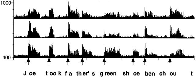
ONSET DETECTION. There is one additional kind of shaping of the acoustic signal that Shamma left out here by choosing the specific example utterance he used. One important property for speech is the onset of vowels. These are distinctively marked in the auditory system (see Port, 2003 J. Phon). If there are abrupt acoustic onsets in lower frequencies in the signal (especially at the onsets of stressed vowels) then there is a nonlinear exaggeration of energy onsets. The figure below (from Delgutte, 1997) show histograms of the firing rate of several cells in the auditory nerve of a cat when presented with an English sentence. The center frequency of the 3 fibers are about 400 Hz, 550 Hz and 790 Hz. Since there is much more energy in low frequencies than high, this makes vowel onsets far more salient than the onset of high-frequency consonant energy. Thus the perceptual onset of syllables like so and shoe is really the vowel onset, not the fricative onset. You can demonstrate this to yourself by making taps line up with regularly syllables: if you slow down and listen closely, you can hear that your taps line up naturally with the vowel onset, not the fricative onset.3. Psychophysics
Psychophysics is the study of the relationship between physical stimulus properties and sensory responses of the human nervous system as reported by subjects in experimental settings. Naturally, auditory psychophysics is specifically concerned with hearing.4. Pattern Learning.
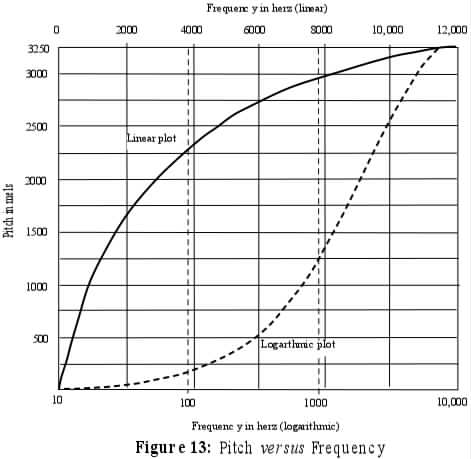
PITCH is a psychological dimension that varies with physical frequency. The relation between perceived pitch and frequency is roughly linear from 20 Hz to about 1000 Hz (thus including the range of F1 but only the lowest part of the range of F2. Thus, to say it is a linear relation is to say that the perceived amount of pitch change between 200 Hz and 300 Hz is the same as the change from 800 Hz to 900 H (both are a difference of 100 Hz). But between 1 kHz and 20 kHz, the relation is logarithmic. Thus the pitch change between 1000 Hz and 1100 Hz (a 10% difference) is about the same as the difference between 5000 Hz and 5500 Hz (also 10% although a 5 times larger change in linear Hz). It is also the same as 12000 Hz and 13200 (10%). THus doubling a 100 Hz tone to 200 Hz is an octave change and very distinctive, but an increase in frequency of 100 Hz beginning at 15 kHz, since it is about 1%, is just barely detectible as any difference at all. There are several technical scales that represent pitch, such as the mel scale and bark scale (which are very similar although defined in different ways), where equal differences represent equal amounts of pitch change. The figure below shows mels on the vertical scale plotted against two different frequency scales. The solid line is labelled across the top in linear Hz and the dotted line is labelled across the bottom in log Hz.
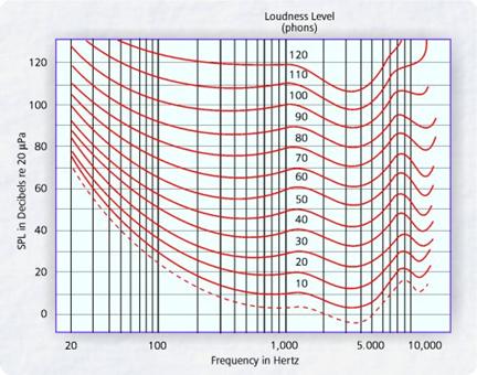
LOUDNESS is a psychological dimension closely related to physical intensity. Below is shown a graph of equal loudness contours on the plane of frequency (displayed as a log scale) against intensity (sound pressure level or dB SPL), a measure of physical energy in sound. The numbers within the graph represent `loudness levels' obtained by playing pure tones at various points in the plane and asking subjects to adjust a 1000 Hz tone to have the same perceived loudness. Notice that for both frequencies below about 300 Hz and frequencies above about 5 kHz, increased intensity is required to have the same loudness as the 1000 Hz tone. (Since gain or loudness knob on a stereo system actually controls intensity, this is why you need to boost the bass on your stereo system if you turn the volume down low: otherwise the lows become inaudible.)
The significance of this graph is that only low frequencies are resolved well. At high frequencies, pitch sensations are scrunched together and only large differences are noticeable. Notice also that musical scales are consistently logarithmic: increasing pitch by one octave doubles the frequency. So the musical scale, where octaves repeat, is like auditory pitch only above about 1000 Hz. Both barks and mels turn out to be interpretable in terms of linear distance along the basilar membrane. That is, listeners' judgments about amount of pitch difference are bascially judgments of distance along the basilar membrane. That is, equal differences in perceived pitch amount to equal distances between their corresponding hair cells along the basical membrane.
.
One surprising property of the auditory system is the neural representation of intensity differences, that is, the neural representation of the dynamic range of sound. As noted, human hearing has a dynamic range of over 100 dB between just detectible and causing discomfort. But individual neural cells have only a very small dynamic range of activation levels between the background-level firing (where there is no signal) and the maximum rate of firing of the cell. So the auditory system has a variety of tricks, some quite complex, to achieve the 100 dB dynamic range.
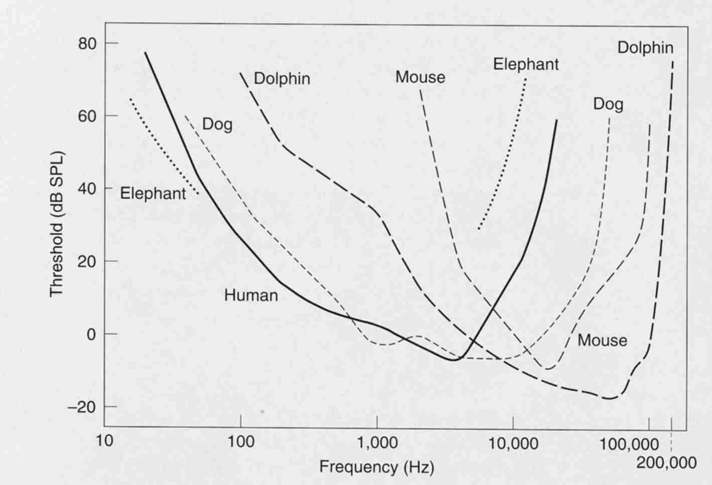
Different animals hear different frequency ranges -- as shown below. Some animals can hear much higher frequencies than humans can while others cannot hear sounds as low as we can. Noticed there is a rough correlation between physical size and the audible frequency range.
So far, we have discussed the way sound is transformed when it is converted to neural patterns and presented to the lowest levels of the brain. Naturally, what really counts for speech is pattern recognition, and the patterns that matter for speech are primarily those due to moving articulatory gestures over time. There are neural systems that are specialized for recognition of time-varying patterns of a very general nature, and gradually, the child develops specialized neural recognizers for the auditory events to which it is repeatedly exposed. This kind of learning seems to be at the level of auditory cerebral cortex in the temporal lobe. This learning is rote and concrete - specified in a space of specific frequencies and temporal intervals. How could such codes develop?
PRESPEECH AUDITION. At birth, the auditory system is much better developed than the visual system. Newborns can recognize their mother's voice language and even her language (spoken by a different voice) while it takes at least 2 months to recognize her face (DeCasper & Fifer, 1980). There is much evidence that the auditory system is quite functional in utero. After all, the fetus has plenty to listen to (even if its low-pass filtered) while it has nothing to see. Successful speech discrimination studies have been done on 4-5 week old infants demonstrating ability to discriminate at least major linguistic sound contrasts: eg, /i/ from /a/, /ba/ from /pa/, etc. There is now a great deal of evidence that during their first year children learn to distinguish the important sound types of their ambient language while learning to ignore differences that are not distinguished in the language they are learning (Werker and Tees, 1984). The allophone-like spectro-temporal trajectories that occur are probably recognized in fragments of various sizes. And any sound patterns that occur very infrequently or are novel tend to be ignored or grouped with near neighbors that do occur frequently. These are the phenomena that have been used to justify `categorical perception,' the `magnet effect,' etc. This clustering process or partial categorization of speech sounds takes place at a time when infants produce no words (which doesn't happen till about 12 mo) and recognize only a small number of them.
Presumably the auditory system develops similarly to the visual system. It is known that development occurs by combining primitive sensory patterns into successively more complex ones. Thus, dots combine into small edge and bar detectors at various spatial scales (from tiny to very large) which combine into large pattern fragments. The main difference between vision and audition here is that visual pattern primitives have 2 spatial axes plus time while audition must be frequency by time. That is, auditory features will be either spectrally static or, more typically, spectrotemporal. The organization and learning processes will be very similar between vision and audition. But there is much less research on audition compared to vision.
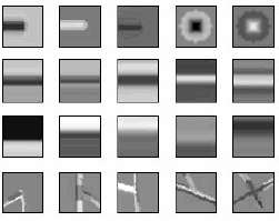
So to illustrate the process from the artificial vision literature, we first need to see how the same pattern features can be found at different spatial scales in the same image. Here are some sinusoidal spatial frequency displays and the receptive fields of simple bar detectors appropriate for each.
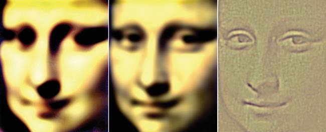
 Here is a visual image filtered to show different spatial frequencies (although the original is not shown). On the left we see only low spatial frequency components of the image (which is fuzzy and lacking in detail), then mid frequencies, and then high frequencies only on the right. The right-hand image shows sharp edges but no large-scale changes in darkness. Notice how looking for, say, edges between light and dark would give you completely different descriptions depending on which image you applied that to. But if you add all three images to each other, the original image would be reconstructed.
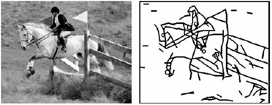
On the left below are some pattern primitives at one spatial scale and one rotational axis (developed by computer vision researchers). To the right, the analysis the bar and edge features are shown for the image in the middle.. Imagine these bar, edge and dot primitives at different spatial scales, each looking for matching patches of the image. Such a description can pick out the major components of a visual pattern.
Returning to audition, imagine a system of similar primitives at different spectrotemporal scales looking for fragments in a static time-slice of the spectrogram-like image like the lower-right blue image in (diii) above. Both the harmonics of a voice fundamental can be captured as well as a formant shapes made from those harmonics (at a larger spatial scale).
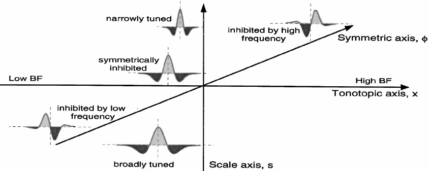
Cortical representation of speech spectral slices (often called spectral profiles), can be encoded using similar descriptors. Shamma proposes that primary auditory cortex (ie, spelled AI but pronounced `A-1') has 3 axes shown below: frequency (the tonotopic axis), tuning width (for wide vs. narrow spectral shape components -- perhaps displayed as depth from the surface of the cortex) and a symmetry axis that distinguishes patterns from strong-weak to balanced (symmetrical) to weak-strong patterns (perpendicular to the tonotopic axis along the surface of AI). These descriptors will capture the main features of any static spectrum.
DYNAMIC CODING. Of course, many of the most important properties of speech signals have not yet been captured since they depend on change in spectral shape over time (eg, formant transitions). Let's call this the speech dynamics layer. These units comprise another layer of cortical cells whose inputs come from the static spectral descriptors of AI (shown above). Thus an isolated rising formant transition will excite a cell that fires only when it gets input from one symmetrical AI cell followed in time by one or several other symmetrical cells to its right along the tonotopic axis. A falling isolated formant (with some particular slope) will be detected by a cell that fires only for a sequence of symmetrical patterns moving left along the frequency axis. This final layer (whose location is not yet known, as far as I know) will provide the kind of description that can be specific to particular syllables. Of course, these cells will self-organize in speaker-hearers for the language to which they are exposed.
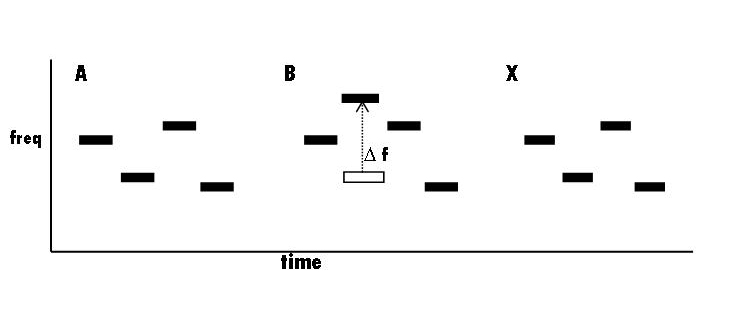
COMPLEX PATTERN AND CATEGORY LEARNING. Speech perception (according to me) is acquired like other complex auditory (or visual) patterns -- by simply storing a great many rather concrete (that is, close-to-sensory) representations of instances or tokens (or exemplars). If a very complex but completely unfamiliar and novel auditory pattern (such as syllables in a language you don't know) is played to an adult, they will be able to recognize very little about it. Why? Because it is complex and matches nothing in memory. But if the complex pattern is repeated many times, eventually, subjects ``construct'' a very detailed description of the pattern. Presumably, this means that some specific cells become tuned to the combination of simpler events from which it is composed. Charles S. Watson (IU Sp & Hrg Dept) has done many experiments using a sequence of 7-10 brief pure tones chosen randomly from a very large set of possible tones. (The example below has only 4 tones.) A complete 10-tone pattern was completed in less than a second. (The patterns sound much like an auto-redialed telephone number.) Such patterns are completely novel and extremely difficult to differentiate from each other or to identify. In many of his experiments, Watson would use the ABX paradigm (see figure below): eg, play a random tone pattern 3 times to a subject and change the frequency of one of the tones between A and B. Then the subject has to say if X, the third repetition, is the same as the first or second (Ie, `Does X match A or B').
If the frequency change is fairly small, subjects do amazingly poorly, compared to what they could do listening to just the changed tone in isolation. However, if a subject is presented the same pattern for many trials (hundreds of them), eventually they learn the details of that pattern and can detect small changes (delta-f) in one of the tones. That is, they will learn a detailed representation for any pattern given enough opportunities to listen to it. Given this amount of training, detecting a frequency change in one component is then almost as easy as detecting the change in a single isolated tone.
Apparently, as we become skilled listeners, we develop feature detectors for, initially, isolated auditory fragments. Gradually, larger spectrotemporal fragments develop from the smaller ones. Some of these fragments (or auditory features) are appropriate for the speech sounds and sound patterns of the ambient language. As we become skilled at speaking our first language, we become effective categorizers of the speech sounds, such as the words and phrases in our language, etc. So abstract categories of speech sound (like syllable-types, letter-like phonemes, etc.) are eventually learned. A category is a kind of grouping of specific phenomena into classes based on some set of criteria. (Of course, a category is only remotely similar to the kind of symbol token assumed to provide the output of the speech perception process by linguists and many psychologists). For one thing, these categories will be distinct for different speaker's voices. Presumably, episodic memory for speech, is based on a code of this sort.
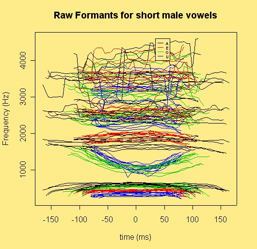
This image shows the formant trajectories of a number of repetitions of the English words dead, Dad, doed, dood as pronounced by an Australian speaker. We should imagine that each of these trajectories is encoded as fragments representing a single formant or several formants plus, of course, the stop burst shapes, etc. We can think of these as an approximation to episodic memory for such words.
Conclusion.
My proposal is that speech perception is based on nonspeech, auditory perception. Each child learns a descriptive system of auditory features that must differ in detail from child to child, since they are independently developed by auditory experience beginning in the womb. This feature system employs both spectral and temporal dimensions. Still, this high-dimensional representation makes it possible to store large numbers of concrete, detailed records of specific utterances. This body of detailed auditory records provides (I think), the database on which linguistic categorization decisions are made.