Gaussian Elimination (LU Factorization) and the BLAS
The most commonly used direct method for solving general linear systems is
Gaussian elimination with partial pivoting, which in modern terms is called LU
decomposition with pivoting, or LU factorization with pivoting. You
probably learned Gaussian elimination by adjoining the right hand side vector b to
the matrix, then performing row combinations that would zero out the subdiagonal
entries of the matrix A. LU decomposition (or "LU factorization") does the same
operations, but ignores the right hand side vector until after the matrix has been
processed. In particular: Let A be an n x n nonsingular matrix. Gaussian
elimination with partial pivoting gives the factorization P*A = L*U, where
- P is a permutation matrix, that is, it has
exactly one 1 in each row and column, and zeros elsewhere.
P-1 = PT,
and can be stored as an integer vector of length n.
Because P-1 = PT,
the factorization can be stated as A = PT*L*U
- L is unit lower triangular matrix (ones on main diagonal,
zero above main diagonal)
- U is upper triangular matrix (zeros below the main diagonal)
The linear system Ax = b then is equivalent to LUx = Pb, since PAx = Pb. Given the
factors P, L, and U, solving LUx = Pb has three steps:
- Set d = Pb, either
by shuffling entries of b, or by accessing via indirect
addressing using a permutation vector.
In setting d = Pb, sometimes b can be overwritten
with its permuted entries ... depending on how P is represented.
- Solve Ly = d (unit lower triangular system)
- Solve Ux = y (upper triangular system)
Solving a triangular system is easy.
It can be implemented by overwriting the right
hand side vector b with the solution, avoiding extra storage for additional vectors
y and d. In that case the three steps look more parsimonious with space:
- Set x = Pb
- Solve Lx = x (unit lower triangular system)
- Solve Ux = x (upper triangular system)
and if the original right hand side vector b is not needed later on,
x can be replaced with b in all three steps.
Warning: the n x n permutation matrix P is not stored as an n x n
array. Instead it is stored as an 1-D integer array, usually called ipiv.
Initially this
will be ignored, and the factorization stated as A = L*U. In this case, what is the
load/store analysis? The minimal number of memory references is n2 words
for A, and n2 for L and U (since L is unit lower triangular, and so the
ones on its main diagonal need not be stored.) That gives m = 2 n2. Later
(after deriving the first version of LU factorization) it can be shown that
the number of flops is f ≈ (2/3) n3.
[The exact count is f = (1/6)*n*(4*n+1)*(n-1), if you want to be precise.]
So the ratio of memory
references to flops is r = 3/n → 0 as n → ∞. That means some
implementation exists for which near peak performance of a computer should be
achieved. The eventual goal is now to find that implementation.
The classical algorithm you probably learned (and may need to unlearn) follows
a four phase sequence on each step: find the ""pivot"", interchange rows to
bring the pivot to the diagonal position, scale the subdiagonal entries
in the column, then update the rest of the matrix.
Omitting the first two steps that implement pivoting,
the process zeros out the subdiagonal elements by adding a multiple of
row k to rows k+1, k+2, ..., n, each step introducing a zero in the elements
A(k+1,k), A(k+2,k), ..., A(n,k). After doing this for the first n-1 rows,
the array A contains the upper triangular
matrix U. The multipliers of row k that were added to the other rows are stored
in the elements A(k+1,k), A(k+2,k), ..., A(n,k) since we know those are zeroed
out. Those multipliers are the strictly lower triangular components of the
unit lower triangular matrix L.
So carrying out these operations with overwriting of the array A gives the L
and U factors in the corresponding
parts of A (since L is unit lower triangular, its diagonal doesn't need
to be explicitly stored, so
everything fits tidily). Temporarily ignoring pivoting, the algorithm is:
for k = 1:n-1
  for i = k+1:n
      A(i,k) = A(i,k)/A(k,k)
  end for
  for i = k+1:n
      for j = k+1:n
        A(i,j) = A(i,j) - A(i,k)* A(k,j)
      end for
  end for
end for
A Matlab function for this is in
LU1.m, but it uses different
index variables (r, c, i) instead of the (k, i, j) shown above.
Notice that the innermost loop (on j) implements a vector update or
daxpy() operation. That makes sense; the algorithm was derived by
adding a multiple of one row to another, which is vector update where
the vectors are the rows of the array A. Load/store analysis says implementing
the algorithm this way gives a ratio of r = 3/2, which is not good.
In fact, although this version is the one most readily derived, it's also the
one that usually has the worst performance.
Matlab notation (AKA colon notation) helps cut down the rat's nest of indices
in the loops:
- A(r:s, i) refers to rows r through s in column i,
- A(r, i:j) refers to columns i through j in row r,
- A(r:s, i:j) refers to rows r through s in columns i through j.
(1) is a column vector, (2) is a row vector, while (3) is a 2D submatrix.
Now the algorithm above can be stated more succintly as
for k = 1:n-1
  A(k+1:n,k) = A(k+1:n,k)/A(k,k)
  A(k+1:n,k+1:n) = A(k+1:n,k+1:n) - A(k+1:n,k) * A(k,k+1:n)
end for
The Matlab function
LU0.m implements this, along with some
error checking to make sure the divisor A(k,k) is not too small, A is square, etc.
This notational change is more important than saving on writing. It
helps identify what the computation kernels are by following three rules
for a 2D array:
- If both the row and column indices have a range, the referrent is a 2D
array (a submatrix)
- If one index has a range and the other is a singleton, the entity is a 1D
array (a vector).
- If neither index has a range, the critter is a scalar.
So in this case, A(k+1:n,k) = A(k+1:n,k)/A(k,k) is the scaling of the
column vector A(k+1:n,k) by the scalar 1/A(k,k). The second line
A(k+1:n,k+1:n) = A(k+1:n,k+1:n) - A(k+1:n,k) * A(k,k+1:n) is
a matrix A(k+1:n,k+1:n) minus the column vector A(k+1:n,k) times the row vector
A(k,k+1:n), or a rank-1 update of a matrix.
The notation can be simplified even more in Matlab (and Fortran)
using indexing vectors :
for k = 1:n-1
    I = k+1:n
    A(I,k) = A(I,k)/A(k,k)
    A(I,I) = A(I,I) - A(I,k)* A(k,I)
end for
The Matlab function
LU2.m implements this but again
with a different loop index r instead of k. The Matlab version also
supresses the printing of every assignment by appending a semicolon
at the end of each assignment operation in the loop.
This follows a useful convention: use upper case letters for vectors used
for indexing (AKA index vectors), and lower case letters for scalars used for indexing.
Using block indexing vectors can sometimes obscure more than it reveals,
so the first form is prefered. Both of the forms
shows more clearly what the operations involved are.
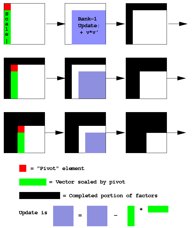
Each iteration is a vector scaling of the subdiagonal part of column k,
followed by a rank-1 update of the trailing part of the matrix.
Graphically, the LU rank-1 update form procedure is:

The rank-1 update version of LU stinks as a computational kernel has a
memory reference to flop ratio of 1. That is better than the 3/2 that results
if it is implemented as a sequence of calls to daxpy(), but we know more
efficient versions must exist.
A more efficient version comes via
a common idea in computer science, where it is called "lazy evaluation".
In numerical linear algebra it has a longer history, and is called
"deferred updates". This means holding off application of the updating
information to a part
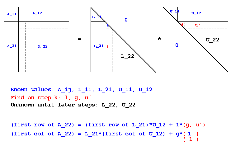
of the matrix only when it is actually needed. The algorithm results by
equating parts of A, L, and U in a partitioned way. In pictures:

The diagonal entry in column k of L is known to be all 1s, of course.
Sequencing the finding of g, u', and l as shown above
defines an algorithm which recursively works on the trailing
subblock. The resulting algorithm is
for k = 1:n-1
   A(k:n,k) = A(k:n,k) - A(k:n,1:k-1)*A(1:k-1,k)
   A(k,k+1:n) = A(k,k+1:n) - A(k,1:k-1)*A(1:k-1,k+1:n)
   A(k+1:n,k) = A(k+1:n,k)/A(k,k)
end for
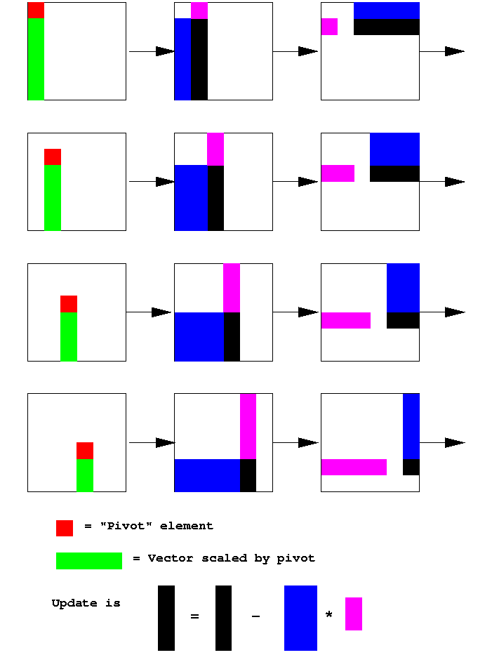
In order the computational kernels in the k-loop are matrix-vector
product,
vector-matrix product, and vector scaling. So the rank-1 update
has been replaced by matrix-vector products, which have half the
memory reference to flop ratio of a rank-1 update. This is a
big win on a cache-based machine.
Minor point performance-wise, but big in terms of correctness:
there is a final update of A(n,n) which has been left off
above. Figure out what it is and correct the algorithm.
In pictures the LU matrix-vector product form procedure is:

Three more notes:
- The algorithms above (rank-1 and matrix-vector product
formulations) can be applied to an m × n rectangular matrix. If m > n,
then L is unit lower trapezoidal and U is upper triangular. If m < n, then
U is upper trapezoidal, and L is unit lower triangular.
- In some literature, the different versions are labeled by the order
of the loops, e.g.,
the kij version,
the jki version, etc. That requires knowing which index variable is
used for which loop in the "original" version, making it harder to
remember. Naming the versions based on their underlying computational
kernels seems more descriptive and mnemonic, and makes shifting them
to use the BLAS easier.
- This page has taken LU factorization from a daxpy() version (r = 3/2), to a
dger() version (r = 1) to a dgemv() version (r = 1/2). The load/store analysis
at the start shows a version exists with r = 0; that will be found after
first dealing with the other parts of solving a linear system, permutations
and triangular solves.
Next: Permutation/pivot vectors and triangular solves
- Started: 23 Aug 2011
- Modified: Wed 24 Sep 2014, 11:18 AM for typos, load/store comments
- Last Modified: Mon 04 Nov 2019, 06:59 AM
