Recall that P is the set of languages that can be decided in deterministic polynomial time and NP is the set of languages that can be decided in non-deterministic polynomial time. Since every non-deterministic Turing machine is also a deterministic Turing machine, P ⊆ NP. It is not know whether P = NP.
We use the terms language and problem interchangeably. The problems that we are interested in are always those that can be answered in “yes” or “no”. Such problems naturally induce a language—the set of inputs for which the answer is “yes” is exactly the language corresponding to that problem.
A specific subset of NP is called NP-complete. A language in NP is NP-complete if every other problem in NP can be reduced to it in deterministic polynomial time. As a consequence if a deterministic polynomial time algorithm is ever discovered for any NP-complete problem then all problems in NP will become solvable in deterministic polynomial time. In other words, the class NP will collapse into P.
If we can prove, from first principles, that one particular problem is NP-complete then we can prove the NP-completeness of several other problems by doing a reduction instead of using the first principles each time. Typically, sat is the starting point for this process, which is proved NP-complete by explicitly constructing a Boolean formula for an arbitrary non-deterministic Turing machine finishes its computation in polynomial time operating on a specific input. The formula is constructed in such a way that it is satisfiable, if and only if, the machine accepts its input. Moreover, the length of the formula is a polynomial in the length of the input to the machine and is constructed in polynomial time. This construction is the proof of Cook's Theorem.
To prove the NP-completeness of any other problem, say P, all we need to do is show that P is in NP and that there is a polynomial-time reduction from a known NP-complete problem to P. Note that the term “reduction” assumes that transformation is correct, in that the solver for P can be correctly used to obtain the solution to the known NP-complete problem that is being reduced to P.
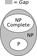
Consider the set NP – P – NPC, where NPC denotes the set of NP-complete problems. Are there any problems that lie in this set? It turns out that most problems that are in NP, but not known to be in P, are NP-complete. However, there are a few that are suspected to be in the gap.
As of 1979 there were three problems that were suspected of falling in this gap.
Each problem is easily shown to be in NP. In 1979, Leonid Khachian came up with a polynomial-time algorithm for linear-programming. So, it proved that the problem was in P. Unfortunately, the algorithm itself was not very fast in practice because it was complicated. In 1984 Narendra Karmarkar described a much more efficient algorithm that worked well in practice. Techniques based on Karmarkar's algorithm are widely used today.
Determining whether a number is prime (equivalently, composite) has fascinated mathematicians for centuries. However, it was not until 2002 that an efficient algorithm was discovered to solve the problem. Manindra Agrawal, Neeraj Kayal, and Nitin Saxena discovered an algorithm in 2002 (complete version published in 2004) that established that the problem of answering whether a given number in binary was prime was in P. Since complement of any language in P is also in P, this implies that composites is in P. Note, however, that this does not solve the problem of actually finding prime factors of a number, which remains a difficult problem to solve and is the basis for many cryptographic methods.
Two graphs are isomorphic if the nodes in one can be renamed to make it identical to the other. A polynomial time algorithm for graph-isomorphism problem still remains elusive. Notice that this problem is different from subgraph-isomorphism in which a graph needs to be isomorphic to a sub-graph of the other. subgraph-isomorphism is NP-complete, as we proved in the last assignment. graph-isomorphism, on the other hand, has not been proved NP-complete. Why does your reduction for subgraph-isomorphism not work for graph-isomorphism? The graph-isomorphism problem is suspected to be somewhat easier than subgraph-isomorphism because we do not have to check isomorphism for each sub-graph of one of the graphs, only between the two graphs.
The list of known NP-complete problems is long and is constantly growing. Several of these problems have other related problems that turn out to be much simpler. Here are some such problems and their simpler counterparts.
If L ∈ P, is L¯ ∈ P? The answer is yes, because given a deterministic polynomial time Turing machine for recognizing L it is easy to construct one that accepts L¯. Simply make all the final states non-final and all the non-final states final. We will also need to make sure that the new machine accepts all the strings on which the original machine crashed. This can be done by completing all the missing transitions in the original machine by having them all go to a non-accepting state, before complementing the machine. This is very similar to what we did to obtain a complement DFA.
The same idea does not work with non-deterministic machines. The reason is that there is an inherent asymmetry in non-deterministic machines. The machine accepts as long as there is one accepting computational path, whereas each computational path has to fail for it to reject. As a result, the polynomial time bound of the computation in the original machine is no longer applicable in the complement machine. Why?
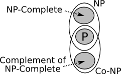
In fact, it is unknown whether or not the complement of NP problems are themselves in NP. The set consisting of the complement of NP problems is called Co-NP. There is certainly some overlap between the two sets. In particular, P ⊆ (NP ∩ Co-NP). Moreover, according to what we know, NP-complete problems do not belong to the intersection and nor do the complements of the NP-complete problems.
The following two theorems, which we state without proof, summarize what is known about these classes.
Sometimes the complexity classes P, NP, and Co-NP are also discussed without invoking the Turing machine model. P refers to polynomial time algorithms, as before. Recall that due to the equivalence of Turing machines and “standard” computers, the polynomial time may also be counted in terms of steps that can reasonably be performed on any computer in a fixed bounded amount of time.
For a problem to be in NP the problem must be divisible into two steps: obtaining a “certificate”, which is a supposed evidence of a solution to the problem; and verifying that the supposed solution is in fact correct. For example, for sat a certificate is a truth assignment, and the verification step is the process of verifying that the truth assignment satisfies the formula. A problem is in NP if its certificate can be verified in polynomial amount of time, but the process of obtaining a certificate may or may not be polynomial. In fact, if the certificate itself can be obtained in polynomial time then the problem is in P. Notice that this characterization of NP is exactly identical to that in terms of a non-deterministic Turing machine, because the Turing machine can simply guess a certificate and then proceed to verify it in polynomial amount of time.
The certificate mentioned above in effect proves that a given input is in the language. Such a certificate is called a qualifying certificate. Thus, languages in the class NP are exactly those for which a qualifying certificate can be verified efficiently. Co-NP languages, on the other hand, are those for which a disqualifying certificate can similarly be verified efficiently. Again, this characterization of Co-NP is exactly equivalent to that in terms of the complement being in NP.
As the above discussion shows, there are decidable problems that are outside NP. However, none of them is provably outside NP—recall that it is unproven whether or not Co-NP is the same as NP. But it is possible to define other complexity classes and there are problems that are provably harder than P.
PSPACE is the set of problems that require no more than polynomial amount of space to be solved. EXPTIME is the class of problems requiring no more than exponential time. The classes are arranged as follows:
P ⊆ NP ⊆ PSPACE ⊆ EXPTIME
It is also known that P ≠ EXPTIME. Thus, at least one subset relation in the above hierarchy is proper, but we do not know which.
Each of these classes have their own sets of complete problems. For example the chess problem asks the question whether, given a board configuration, the current player can win the game. It turns out that this problem is EXPTIME-complete. Thus, chess is provably harder than P. Unsurprisingly, most multi-player games are very difficult. One exception is sudoku, in which we ask whether given a puzzle and the rules of the game there is a solution. Sudoku is NP-complete.
Any problem that is at least as hard as any NP problem is said to be NP-hard. Thus problems in PSPACE and EXPTIME are NP-hard. Just as completeness can be associated with any problem class, so can be hardness.
Just because a problem is hard does not mean that practical solutions cannot be found. We are often faced with provably hard problems that have to be solved. A simple example is classroom scheduling. Indeed, the list of NP-complete problems is so long precisely because they appear in so many practical situations. In practice there are two common ways to solve the hard problems:
Another strategy that is often employed in practice is based on randomized algorithms, where the algorithm proceeds probabilistically.