Divide and Conquer
B403: Introduction to Algorithm Design and Analysis
Divide and Conquer
- Idea
- Divide the problem into a number of smaller subproblems
- Conquer the subproblems by solving them recursively
- Combine the solutions to the subproblems into the solution of the original problem
- Leads naturally to recursion
- Recursive case: solving subproblems recursively when they are big enough
- Base case: solving a small problem directly
Recurrences
- Result directly from divide-and-conquer algorithms
- Recall Merge-Sort
T(n) = { Θ(1) if n = 1 2T(n/2) + Θ(n) if n > 1
Solving Recurrences
- Substitution method: guess a bound and use mathematical induction to prove it is correct
- Recursion-tree method: convert the recurrence into a tree whose nodes represent costs incurred at various levels of the recursion
- Master method: recipe for solving recurrences of the form
T(n) = aT(n/b) + f(n)
where a ≥ 1, b > 1, and f(n) is a given function
- Note: we often ignore certain technicalities
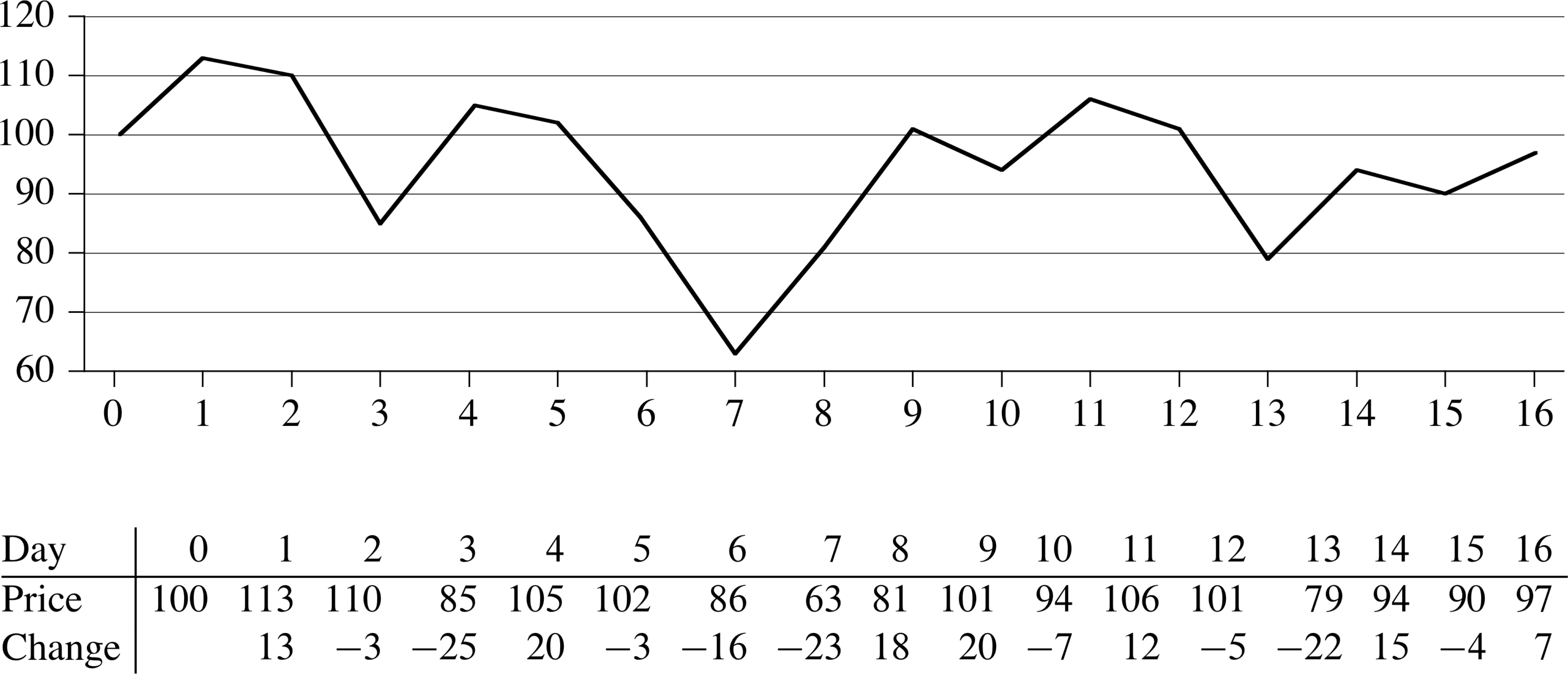
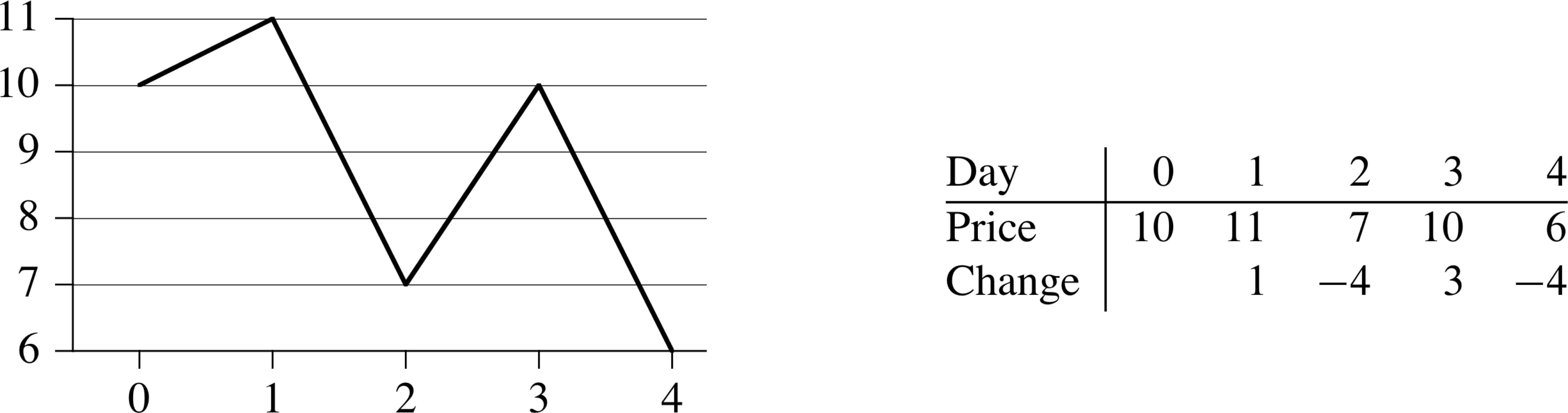
Volatile Chemicals
Given stock prices into the future, allowed to make one purchase and one sale, maximize profit
Volatile Chemicals
Given stock prices into the future, allowed to make one purchase and one sale, maximize profit
What would be a brute-force method?
Maximum-subarray Problem
- Define a new array of size n−1 of daily changes
- Find the contiguous subarray with the largest sum
Will this solve the same problem?
Observation
Any contiguous subarray A[i..j] of A[low..high] must lie in exactly one of the following places:
- entirely in the subarray A[low..mid], so that low ≤ i ≤ j ≤ mid,
- entirely in the subarray A[mid+1..high], mid < i ≤ j ≤ high, or
- crossing the midpoint, so that low ≤ i ≤ mid ≤ j ≤ high
Find Max Crossing Subarray
   Find-Max-Crossing-Subarray (A, low, mid, high)

   1  left-sum = −∞
   2  sum = 0
   3  for i = mid downto low
   4    sum = sum + A[i]
   5    if sum > left-sum
   6       left-sum = sum
   7       max-left = i
   8  right-sum = −∞
   8  sum = 0
   10 for j = mid+1 to high
   11   sum = sum + A[j]
   12   if sum > right-sum
   13      right-sum = sum
   14      max-right = j
   15 return (max-left, max-right, left-sum + right-sum)
Maximum Crossing Subarray: Example
| 1 | 2 | 3 | 4 | 5 | 6 | 7 | 8 | 9 | 10 |
| −10 | 5 | 3 | −4 | 2 | −3 | 7 | 1 | 2 | −5 |
|---|
|
|
Find Maximum Subarray
   Find-Maximum-Subarray (A, low, high)

   1  if high == low
   2    return (low, high, A[low])
   3  else mid = floor((low+high)/2)
   4    (left-low, left-high, left-sum) =
           Find-Maximum-Subarray(A,low,mid)
   5    (right-low,right-high,right-sum) =
           Find-Maximum-Subarray(A,mid+1,high)
   6    (cross-low,cross-high,cross-sum) =
           Find-Crossing-Subarray(A,low,mid,high)
   7  if left-sum ≥ right-sum and left-sum ≥ cross-sum
   8    return (left-low, left-high, left-sum)
   9  elseif right-sum ≥ left-sum and right-sum ≥ cross-sum
   10   return (right-low, right-high, right-sum)
   11 else return (cross-low, cross-high, cross-sum)
Matrix Multiply
  Square-Matrix-Multiply (A, B)
  1  n = A.rows
  2  let C be a new n×n matrix
  3  for i = 1 to n
  4    for j = 1 to n
  5      cij = 0
  6      for k = 1 to n
  7        cij = cij + aik.bkj
  8  return C
What is the time complexity?
Answer: Θ(n3)
Can we do better?
Multiplying using Sub-matrices
|
|
|
Recursive Version
  Square-Matrix-Multiply-Recursive (A, B)
  1  n = A.rows
  2  let C be a new n×n matrix
  3  if n == 1
  4    c11 = a11.b11
  5  else partition A, B, and C into A11, A12, A21, A22, etc.
  6    C11 = Square-Matrix-Multiply-Recursive(A11, B11)
          + Square-Matrix-Multiply-Recursive(A12, B21)
  7    C12 = Square-Matrix-Multiply-Recursive(A11, B12)
          + Square-Matrix-Multiply-Recursive(A12, B22)
  8    C21 = Square-Matrix-Multiply-Recursive(A11, B11)
          + Square-Matrix-Multiply-Recursive(A22, B21)
  9    C22 = Square-Matrix-Multiply-Recursive(A21, B12)
          + Square-Matrix-Multiply-Recursive(A22, B22)
  10 return C
Recursive Matrix Multiply Running Time
| T(1) | = | Θ(1) |
| T(n) | = | Θ(1) + 8T(n/2) + Θ(n2) |
| = | 8T(n/2) + Θ(n2) |
| T(n) = { | Θ(1) | if n = 1 |
| 8T(n/2) + Θ(n2) | if n > 1 |
Strassen's (Straßen's) Method
Idea:
- Set up some intermediate matrices, to reduce the number of recursions from 8 to 7
- Add some Θ(n2) work to remove one recursive call
S Sub-matrices
| S1 | = | B12 − B22 | S2 | = | A11 + A12 | |
| S3 | = | A21 + A22 | S4 | = | B21 − B11 | |
| S5 | = | A11 + A12 | S6 | = | B11 + B22 | |
| S7 | = | A12 − A22 | S8 | = | B21 + B22 | |
| S9 | = | A11 − A21 | S10 | = | B11 + B12 |
P Sub-matrices
| P1 | = | A11 ⋅ S1 |
| P2 | = | S2 ⋅ B22 |
| P3 | = | S3 ⋅ B11 |
| P4 | = | A22 ⋅ S4 |
| P5 | = | S5 ⋅ S6 |
| P6 | = | S7 ⋅ S8 |
| P7 | = | S9 ⋅ S10 |
Compute C using P Sub-matrices
| C11 | = | P5 + P4 − P2 + P6 |
| C12 | = | P1 + P2 |
| C21 | = | P3 + P4 |
| C22 | = | P5 + P1 − P3 − P7 |
You are not expected to remember this, nor are you expected to know how to derive this. However, it is important to remember that Strassen's algorithm is the best known algorithm for matrix multiplication, asymptotically. It is also instructive to see how it achieves asymptotically better performance than standard matrix multiply. In practice, due to the critical impact of memory caches and data locality on modern machines Strassen's algorithm does not perform as well as some other “blocked” algorithms for matrix multiply that are Θ(n3). This is a good example of a situation where a simple asymptotic complexity analysis does not lead to a good insight into the real-world behavior of an algorithm.
Recurrences: We Focus on Master Method
- Substitution method: guess a bound and use mathematical induction to prove it is correct
- Recursion-tree method: convert the recurrence into a tree whose nodes represent costs incurred at various levels of the recursion
- Master method: recipe for solving recurrences of the form
T(n) = aT(n/b) + f(n)
where a ≥ 1, b > 1, and f(n) is a given function
Theorem: Master Theorem
Let a ≥ 1 and b > 1 be constants, let f(n) be a function, and let T(n) be defined on the nonnegative integers by the recurrence:
T(n) = a T(n/b) + f(n)
-
If f(n) = O(nlogba−ε) for some constant
ε > 0, then
T(n) = Θ(nlogba)
-
If f(n) = Θ(nlogba), then
T(n) = Θ(nlogba log n) = &Theta(f(n) log n)
-
If f(n) = Ω(nlogba+ε), for some
constant ε > 0, and
if a f(n/b) ≤ c f(n) for some constant c < 1 and all sufficiently large n thenT(n) = Θ(f(n))
Master Method: Important Special Case
An important special case is when f(n) = ck for some k. In other words, f(n) is a polynomial function.
It turns out that the “regularity condition” (the extra condition for case 3) always holds when f(n) is a polynomial. So there is no need to check for it explicitly.
How would you prove this?
Final Remarks
- The best known square matrix-multiply algorithm to date is O(n2.376), by Coppersmith and Winograd
- The lower bound on matrix-multiply is Ω(n2) Why?
- Reasons for not using Strassen's algorithm, in practice
- larger constant factor hidden in O(nlog 7) than the constant factor in O(n3) in standard square matrix multiply
- Specialized sparse matrix algorithms are faster
- Numerically less stable
- Extra space, and consequently poorer cache behavior
Note that matrix-multiply can also use a mix of techniques, which ameliorates most of the shortcomings of Strassen's algorithm. For example, by using Strassen's algorithm only for dense square matrices, and using standard version for matrix sizes below a certain threshold.
Be particularly careful in checking for the extra “regularity condition” for case 3 in master method. However, if f(n) is a polynomial then, as mentioned on the previous slide, the regularity condition follows automatically.