Sorting and Order Statistics
B403: Introduction to Algorithm Design and Analysis
Heapsort
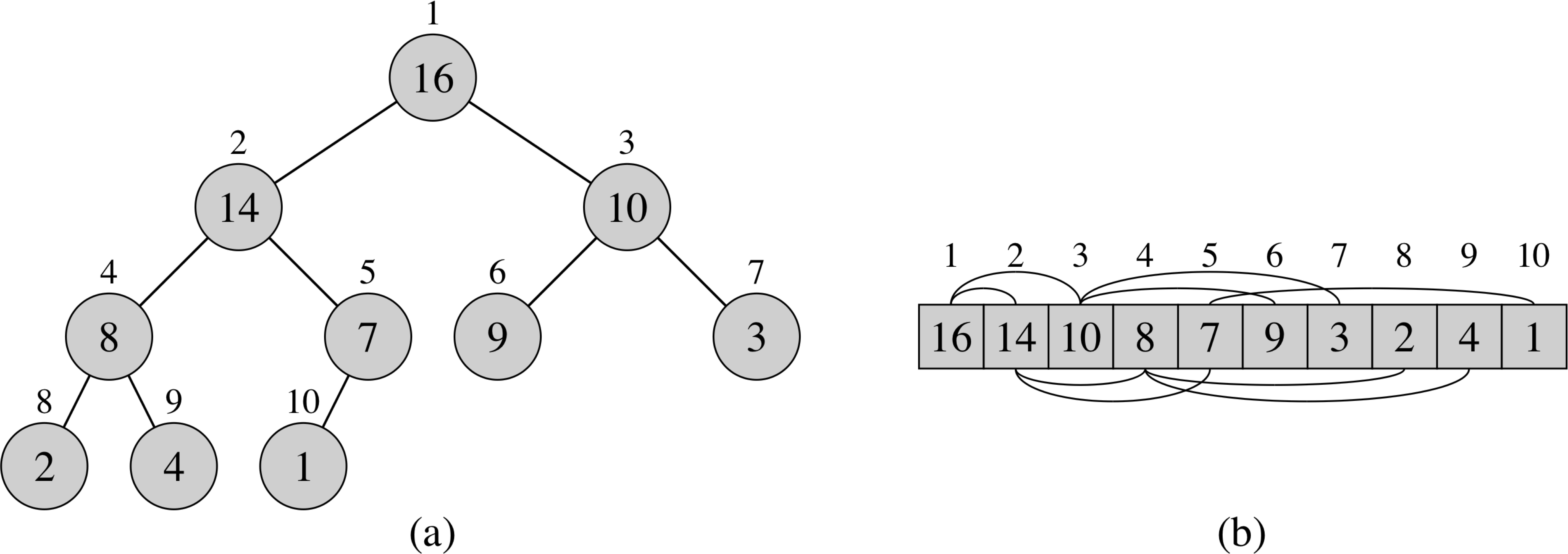
Basic Operations
   Parent (i)

   1  return floor(i/2)
   Left  (i)

   1  return 2i
   Right (i)

   1  return 2i+1
Max-Heap: A[Parent(i)] ≥ A[i]
Min-Heap: A[Parent(i)] ≤ A[i]
Heapify
  Max-Heapify (A, i)

  1   l = Left(i)
  2   r = Right(i)
  3   if l ≤ A.heap-size and A[l] > A[i]
  4     largest = l
  5   else largest = i
  6   if r ≤ A.heap-size and A[r] > A[largest]
  7     largest = r
  8   if largest ≠ i
  9     exchange A[i] with A[largest]
  10   Max-Heapify(A, largest)
T(n) ≤ T(2n/3) + Θ(1)
T(n) = O(log n) (case 2 of master theorem)
Sorting with Max-Heap
  Build-Max-Heap (A)
  1   A.heap-size = A.length
  2   for i = floor(A.length/2) downto 1
  3     Max-Heapify(A, i)
Running time = O(n)
  Heapsort (A)
  1   Build-Max-Heap(A)
  2   for i = A.length downto 2
  3     exchange A[1] with A[i]
  4     A.heap-size = A.heap-size − 1
  5     Max-Heapify(A, 1)
Running time = O(n⋅log n)
Priority Queues with Heaps
  Heap-Maximum (A)
  1   return A[1]
Running time = O(1)
  Heap-Extract-Max (A)
  1   if A.heap-size ≤ 1
  2     error "heap underflow"
  3   max = A[1]
  4   A[1] = A[A.heap-size]
  5   A.heap-size = A.heap-size − 1
  6   Max-Heapify(A, 1)
  7   return max
Running time = O(log n)
Quicksort
Idea: Using divide and conquer
-
Divide: Partition the array A[p..r] into two subarrays A[p..q−1 and A[q+1..r] such that:
A[p..q-1] ≤ A[q] ≤ A[q+1..r]
- Conquer: Sort the two subarrays A[p..q-1] and A[q+1..r]
- Combine: Nothing to be done!
  Quicksort (A, p, r)
  1   if p ≤ r
  2     q = Partition(A, p, r)
  3     Quicksort(A, p, q-1)
  4     Quicksort(A, q+1, r)
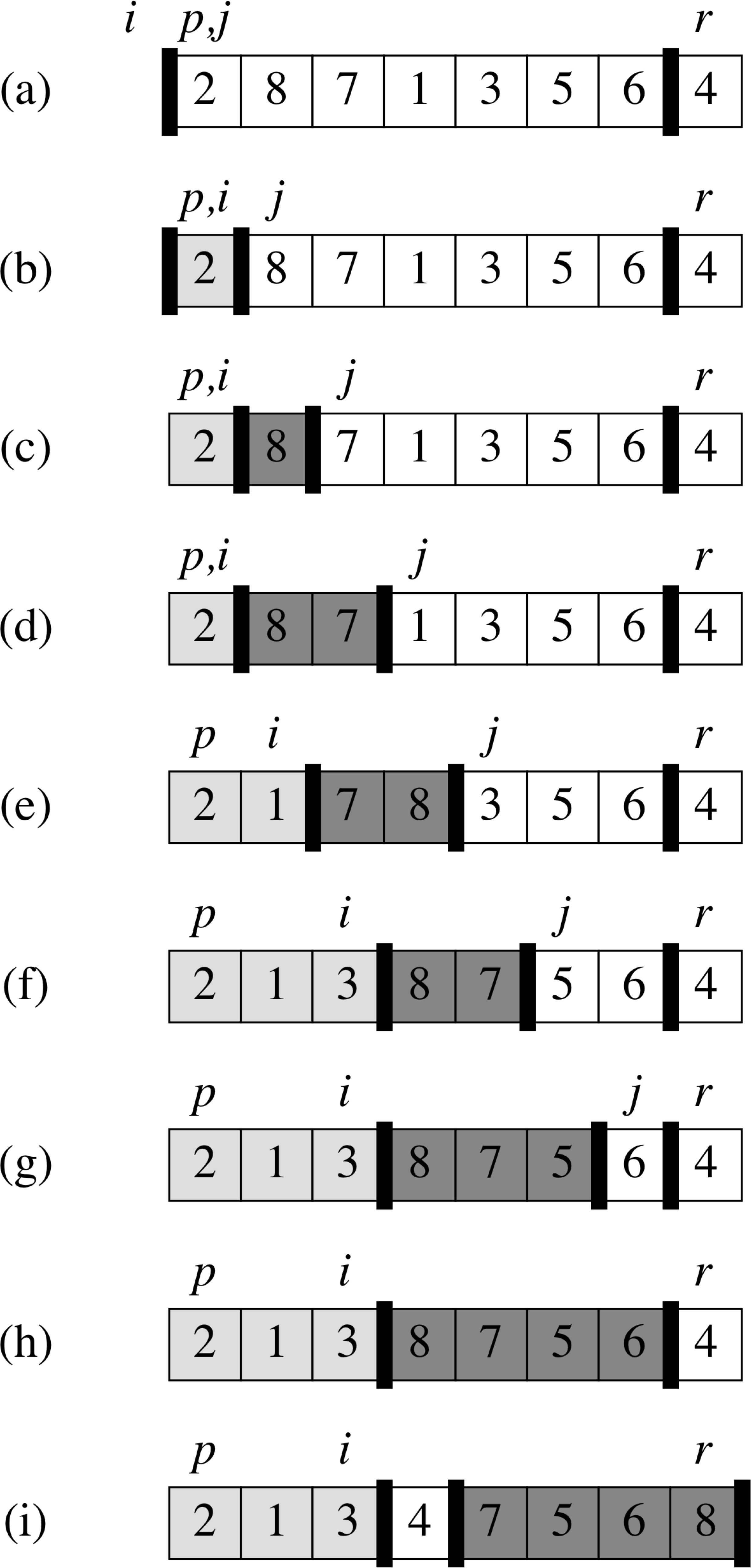
Partitioning the Array
  Partition(A, p, r)

  1   x = A[r]
  2   i = p−1
  3   for j = p to r−1
  4      if A[j] ≤ x
  5         i = i + 1
  6         exchange A[i] with A[j]
  7   exchange A[i+1] with A[r]
  8   return i+1
Partitioning Example
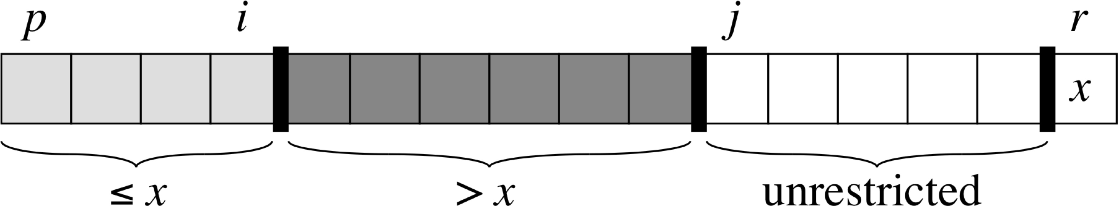
Loop Invariant for Partition
- if p ≤ k ≤ i, then A[k] ≤ x
- if i+1 ≤ k ≤ j−1, then A[k] ≥ x
- if k = r, then A[k] = x
Performance
-
Worst-case partitioning
T(n) = T(n−1) + T(0) + Θ(n) = T(n−1) + Θ(n) T(n) = Θ(n2)
-
Best-case partitioning
T(n) = 2 T(n/2) + Θ(n)
T(n) = Θ(n⋅log n)
-
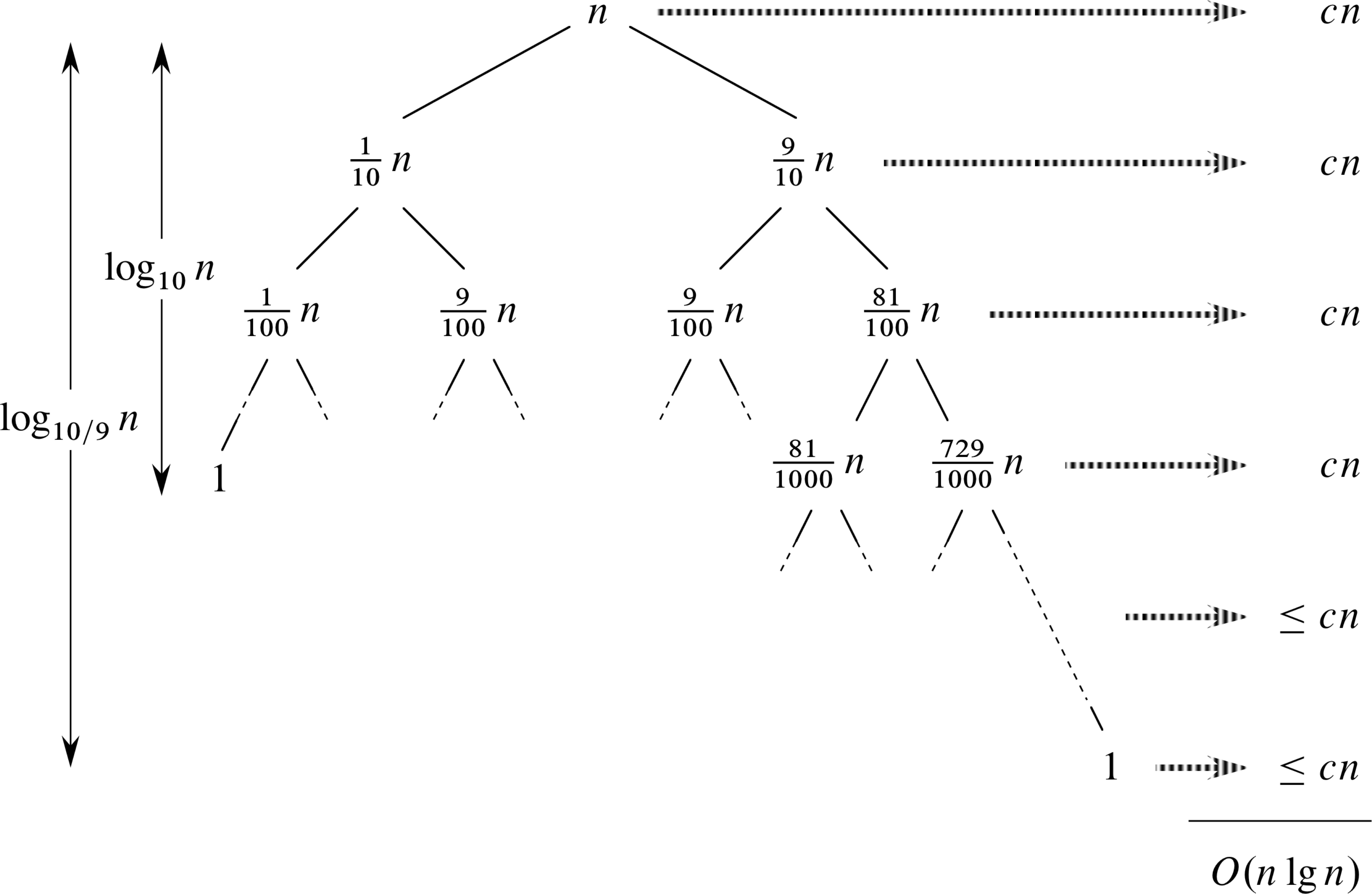
Balanced partitioning
Consider 9-to-1 proportional split at every level
T(n) = T(9n/10) + T(n/10) + Θ(n)
Performance (contd)
Randomized Quicksort
  Randomized-Partition(A, p, r)

  1   i = Random(p, r)
  2   exchange A[r] with A[i]
  3   return Partition(A, p, r)
  Randomized-Quicksort (A, p, r)
  1   if p ≤ r
  2     q = Randomized-Partition(A, p, r)
  3     Randomized-Quicksort(A, p, q-1)
  4     Randomized-Quicksort(A, q+1, r)
Why is this better?
Quick Digression: Indicator Random Variables
| I{A} = { | 1 | if A occurs |
| 0 | if A does not occur |
Lemma: Given a sample space S and an event A in the sample space S, let XA = I{A}. Then E[XA] = Pr{A}.
Proof:
| E[XA] | = | E[I{A}] |
| = | 1⋅Pr{A} + 0⋅Pr{A} | |
| = | Pr{A} |
Lemma
  Partition(A, p, r)

  1   x = A[r]
  2   i = p−1
  3   for j = p to r−1
  4      if A[j] ≤ x
  5         i = i + 1
  6         exchange A[i] with A[j]
  7   exchange A[i+1] with A[r]
  8   return i+1
Lemma Let X be the number of comparisons performed in line 4 of Partition over the entire execution of Quicksort on an n-element array. Then the running time of Quicksort is O(n+X).
Proof: The algorithm makes at most n calls to Partition, each of which does a constant amount of work and then executes the for loop some number of times. Each iteration of the for loop executes line 4.
Computing X
Rename the elements of A as z1, z2, ..., zn, where zi is the ith smallest number.
Define the set Zij = {zi, zi+1, ..., zj}
Each pair of elements is compared at most once
Analyzing Quicksort
Idea: Define an indicator random variable and compute its expected value
| X | = | I {zi is compared to zj} | |
| X | = | n-1 Σ i=1 n Σ j=1+1 | Xij |
| E[X] | = | E[...] | |
| = | n-1 Σ i=1 n Σ j=1+1 | E[Xij] | |
| = | n-1 Σ i=1 n Σ j=1+1 | Pr{zi is compared to zj} | |
Analyzing Quicksort
Observations:
- zi and zj are compared if and only if the first element to be chosen as a pivot from Zij is either zi or zj
- The whole set Zij must be together in a partition before an element from Zij is chosen as a pivot
- Since any element is equally likely to be chosen as a pivot, the probability of choosing any particular element as a pivot is 1/(j−1+1)
| Pr{zi is compared to zj} | = | Pr{zi or zj is the first pivot} |
| = | Pr{zi is the first pivot} + Pr{zj is the first pivot} | |
| = | 2 j−i+1 |
E[X] = n-1 Σ i=1 n Σ j=1+1 2 j−i+1 = O(n⋅log n)
Lower Bound on Comparison Sort
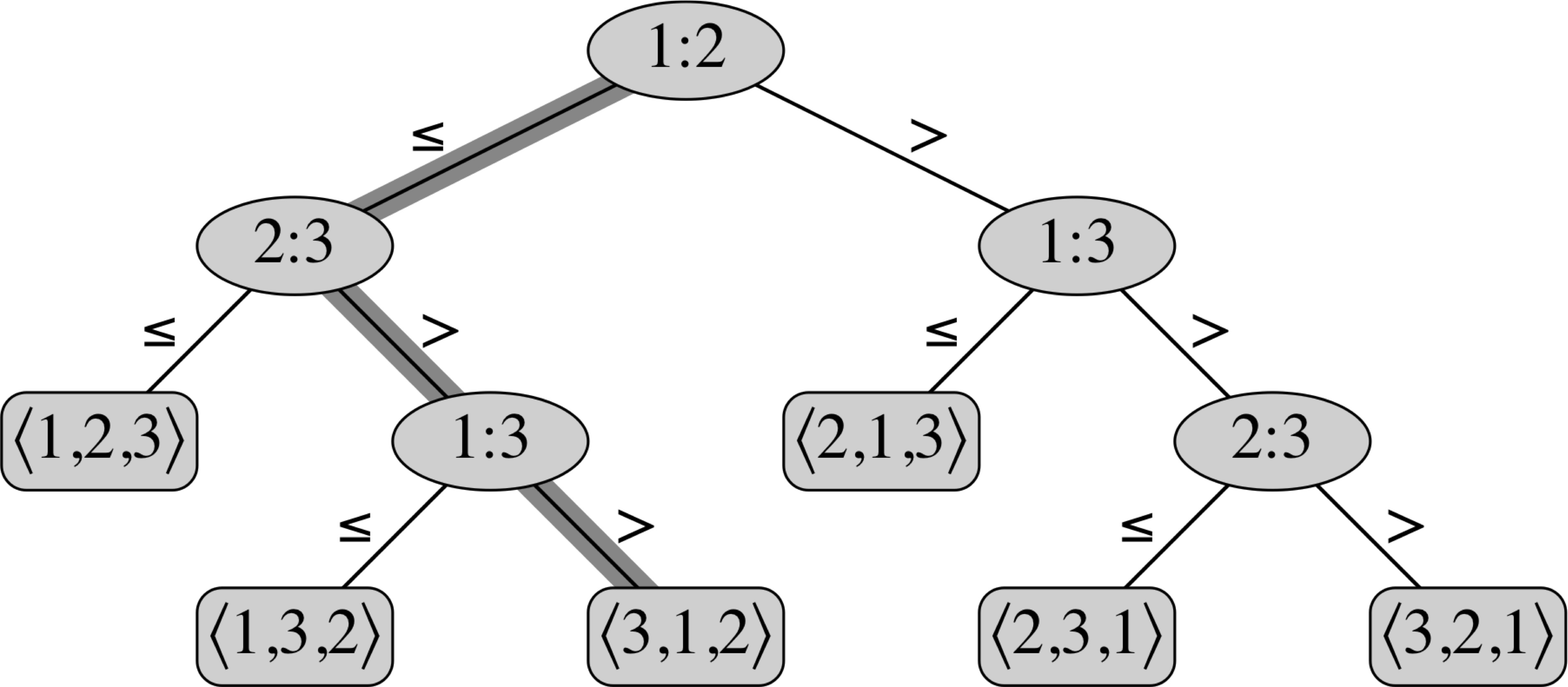
Theorem: Any comparison sort algorithm requires Ω(n⋅log n) comparisons in the worst case.
Proof: We need to determine height of a decision tree in which each permutation appears as a reachable leaf. Consider a decision tree of height h with l leaves. We have:
n! ≤ l ≤ 2h
h ≥ log(n!) = Ω(n⋅log n)
Sorting in Linear Time
- Counting sort
- Radix sort
- Bucket sort
Order Statistic
Input: A set A of n (distinct) numbers and an integer i, with 1 ≤ i ≤ n
Output: The element x ∈ A that is larger than exactly i − 1 other elements of A
Selection in Expected Linear Time
  Randomized-Select(A, p, r, i)

  1   if p == r
  2      return A[p]
  3   q = Randomized-Partition(A, p, r)
  4   k = q − p + 1
  5   if i == k
  6      return A[q]
  7   elseif i < k
  8      return Randomized-Select(A, p, q−1, i)
  9   else
         return Randomized-Select(A, q+1, r, i−k)
Running Time
Let T(n) be a random variable denoting the running time on an input of array A[p..r] of n elements
Since Randomized-Partition is equally likely to return any element as the pivot, for each k such that 1 ≤ k ≤ n, the subarray A[p..q] has k elements (all less than or equal to the pivot) with probability 1/n
Xk = I {the subarray A[p..q] has exactly k elements}
E[Xk] = 1/n, assuming the elements are distinct
For a give call of Randomized-Select, Xk has value 1 for exactly one value of k
Running Time (contd)
When Xk = 1, the two subarrays on which we might recurse have sizes k−1 and n−k.
Assuming that T(n) is monotonically increasing:
| T(n) | ≤ | Σ n k=1 Xk⋅(T(max(k−1, n−k)) + O(n)) |
| = | Σ n k=1 Xk⋅T(max(k−1, n−k)) + O(n) |
| E[T(n)] | ≤ | Σ n k=1 E[Xk⋅T(max(k−1, n−k))] + O(n) |
| = | Σ n k=1 E[Xk]⋅E[T(max(k−1, n−k))] + O(n) | |
| = | Σ n k=1 (1/n)⋅E[T(max(k−1, n−k))] + O(n) | |
| = | Σ n-1 k=floor(n/2) (2/n)⋅E[T(k)] + O(n) | |
| = | O(n) |
Selection in Worst-case Linear Time
Algorithm Select
- Divide the n elements into ⌊n/5⌋ groups of 5 elements each and at most one group of n mod 5 elements
- Find the median of each of ⌈n/5⌉ groups in constant time
- Use Select recursively to find the median of the ⌈n/5⌉ medians found in step 2
- Partition the input array around the median-of-medians x; let x be the kth smallest element, so that there are k-1 elements on the low side and n-k elements on the high side of the partition
- if i = k then return x; otherwise, use Select recursively to find the ith smallest element on the low side if i < k, or the (i−k)th smallest element on the high side if i > k
Why is it Linear?
Linear Time Bound
| T(n) = { | O(1) | if n < 140 |
| T(⌈n/5⌉) + T(7n/10 + 6) + O(n) | if n > 140 |
This results in:
T(n) = O(n)